Accelerating 3D CT Reconstruction using GPGPU

Saoni Mukherjee, Nicholas Moore*, James Brock*, and Miriam Leeser

*: This research was done when Nicholas and James were PhD students at Northeastern University.

Overview

This project accelerates Computed Tomography (CT) reconstruction using GPUs. Acceleration can be beneficial for biomedical image reconstruction applications with large datasets. Graphic Processing Units (GPUs) are particularly useful in this context as they can produce high fidelity images rapidly. An image algorithm to reconstruct cone beam computed tomography using two dimensional projections is implemented using GPUs. The implementation takes slices of the target, weighs the projection data, filters the weighted data to backproject the data, and creates the final three dimensional reconstructions. This is implemented on two types of hardware: CPU and a heterogeneous system combining CPU and GPU. The implementations are based on J. A. Fessler's Image Reconstruction Toolbox [6]. The CPU codes in C and MATLAB are compared with the heterogeneous versions written in CUDA-C and OpenCL. The relative performance is tested and evaluated on mathematical phantoms. Software download information is available here.

Background

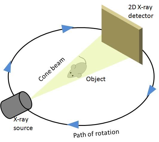
CT reconstruction is a very popular medical diagnostic tool. It provides noninvasive quantification of the human body or living parts for biomedical diagnosis, treatment and research. In a conventional 3D CT setup, the target is placed at the center of an orbital path and the scanner moves around the target taking an image from every possible angle. It produces a set of projections P₁,P₂,..., P_K at K discrete positions of the source with uniform angular spacing. The 2D detector which acts as a sensor stays perpendicular to the axis of rotation and opposite to the x-ray source. Generally the set of source and sensor complete a full 3600 rotation, but sometimes due to mechanical limitations, a full rotation around the target cannot be completed. The collected 2D projections are then reconstructed to produce a cross-sectional view which then forms part of the final 3D volume.

Algorithm

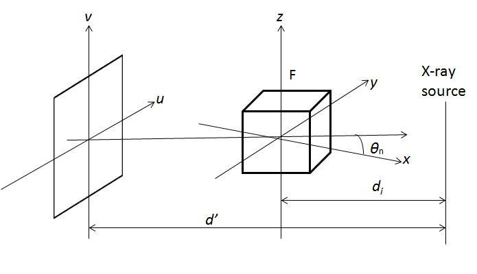
The most famous algorithm for CT reconstruction has been proposed by Feldkamp, Davis and Kress in 1984. This is commonly known as the FDK algorithm; most commercial CT scanners use this. The raw projections P₁, P₂,..., P_K are individually weighted and ramp filtered. Weighting includes cosine weighting and short-scan weighting. The filtered projections are reconstructed to get the final volume. The reconstruction is conceptualized as a weighted backprojection. It is carried out in two stages. In the initial step, the raw data is individually weighted and ramp filtered to produce filtered projections Q₁, Q₂,..., Q_K. The projections are collected at a distance d₀ with angle Theta_n where 1 <= n <= K. d_i is the distance between the volume origin and the source. Let F(x, y, z) denote the value of voxel (x, y, z) in volume F, as shown in the figure above. The xyz space is the volume and uv represents the projections that are to be backprojected to the volume. In backprojection, the volume F is reconstructed using the following equations:

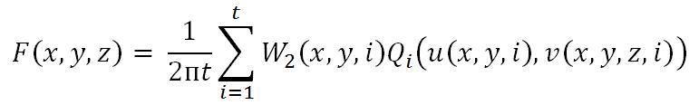
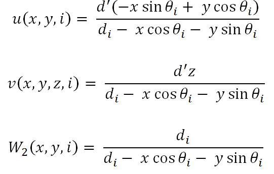
where W₂(x,y,n) represents the weight value and u(x,y,n) and v(x,y,z,n) represent the co-ordinates, which are given by,

                               

Implementation

Among the three steps in reconstruction, backprojection is the most computationally intensive part and takes the most time. However, from the equations mentioned above, it is clear that each voxel is independent of the others. Different voxels can be computed simultaneously. Graphics processing units are especially useful in this context as they provide a massively parallel architecture with hundreds of cores and thousands of threads. For problems that exhibit a great deal of parallelism, the peak performance of GPUs frequently significantly outperforms that of CPUs.

We have divided the total computation in three parts: weighting, filtering and backprojection. Each step is implemented within separate kernels that are launched in a non-blocking manner but executed in series. Note that the complete projection data is moved to GPU memory before any kernel starts execution; after all the kernels complete execution the reconstructed volume is transferred back to the host CPU. This minimizes the expensive cost of memory transfer between host and device.

Architectures used for evaluation

We have tested our GPU implementations in CUDA and OpenCL with serial MATLAB and serial C as well as parallel implementations of C (C with OpenMP constructs) and MATLAB (MATLAB with PCT constructs). The architectures we used are:

Hosts	Devices	Languages
Intel Core i7 quad-core processor @3.4 GHz		MATLAB MATLAB PCT
Intel Xeon W3580 quad-core processor @3.33 GHz	NVIDIA Tesla C2070	C C with OpenMP CUDA
Intel Xeon E5520 quad-core processor @2.27 GHz	AMD Radeon HD 5870	OpenCL

Datasets used for evaluation

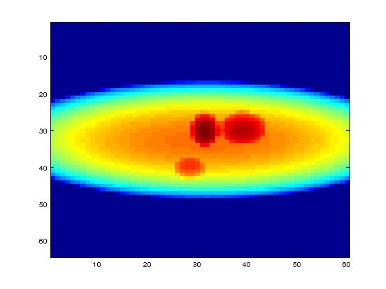
We have used mathematical phantoms generated by MATLAB. One of the mathematical phantoms shown in the picture below is of size
Input: 64 × 60 pixels with 72 projections,
Final volume: 64 × 60 × 50 voxels

Also we have used a mouse scan data of size:
Input: 512 × 768 pixels with 361 projections
final volume: 512 × 512 × 768 voxels
Note that the backprojection code depends on the size of the data, not the content.

Results

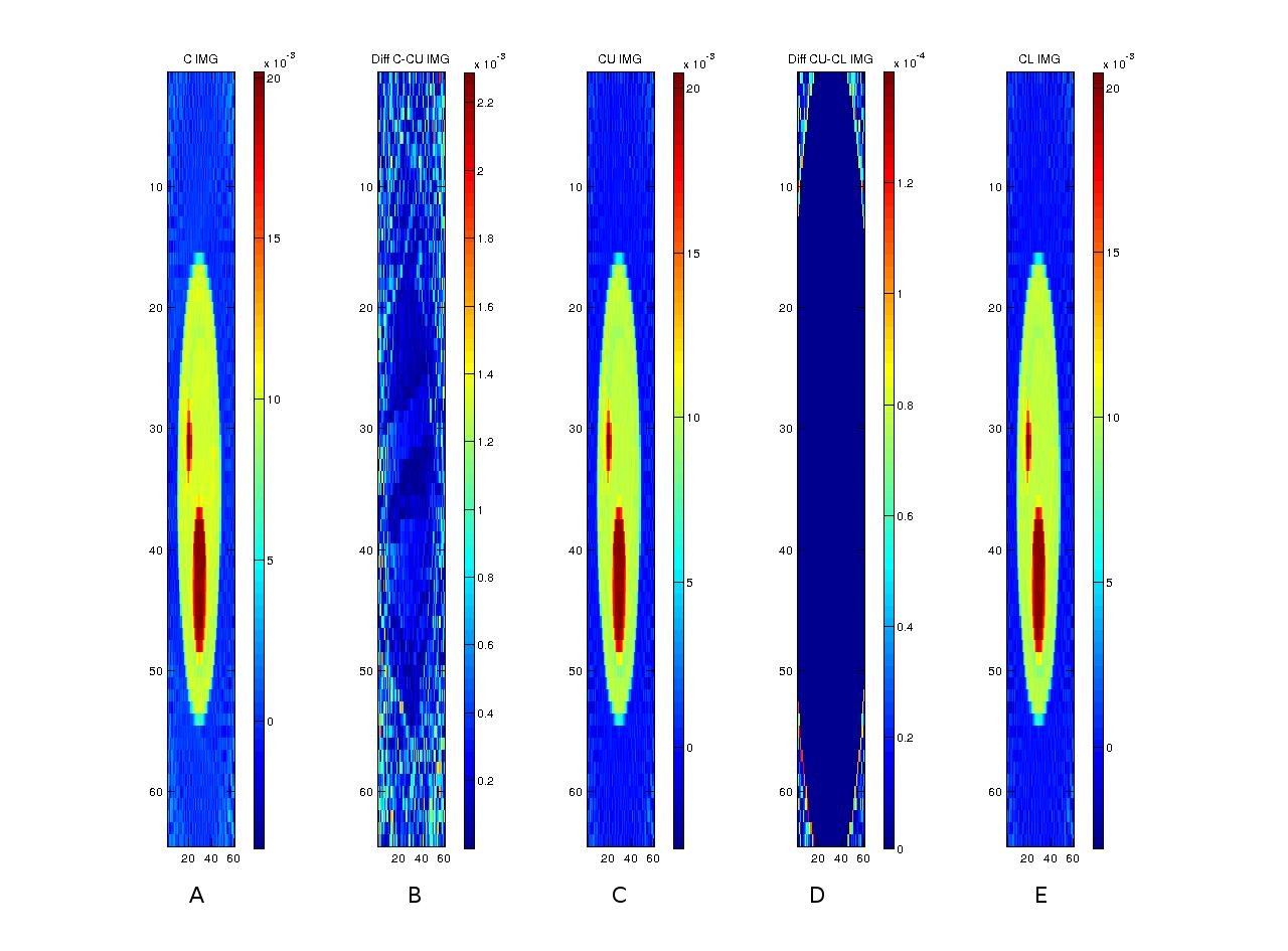
After reconstructing the images, the following shows a comparison of three implementations (in C, CUDA and OpenCL) along with comparisons among the implementations.

A = The image generated by C implementation, C = The image generated by CUDA-C implementation, E = The image generated by OpenCL implementation, B = The difference between the C and CUDA implementations, D = The difference between the CUDA-C and OpenCL implementations.

The following graphs show relative performance of several implementations. The first shows the running time (both total time and backprojection time) of several implementations and the next shows the same in logarithmic scale for the following dataset.

Input: 64 x 60 pixels with 72 projections
Final volume: 64 x 60 x 50 voxels

   

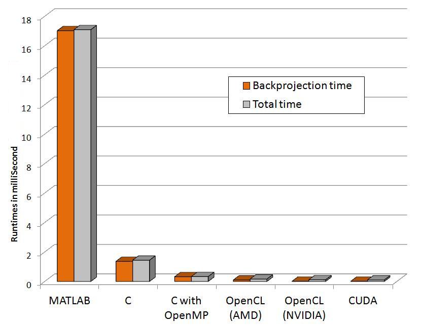
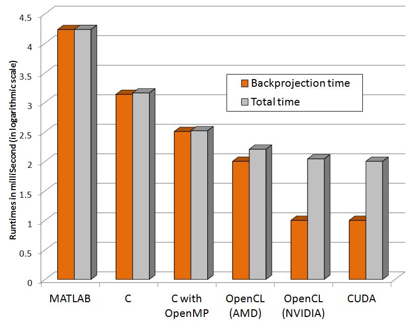
Programming paradigms	Time to run Backprojection (Seconds)	Total time (Seconds)
MATLAB	17.02	17.09
C	1.36	1.44
C with OpenMP (4threads)	0.32	0.33
OpenCL (AMD)	0.10	0.16
OpenCL (NVIDIA)	0.01	0.11
CUDA	0.01	0.10

For the bigger dataset with the mouse scan, the relative performance along with the architecture we used to evaluate is shown. The dataset has:

Input: 512 x 768 pixels with 361 projections
Final volume: 512 x 512 x 768 voxels

Programming paradigms	Hardware	Time to run Backprojection	Total time
MATLAB	Intel Core i7	2h 20m 40s	2h 20m 43s
MATLAB PCT (8threads)	Intel Core i7	1h 32m 36s	1h 32m 39s
C	Intel Xeon W3580	1h 14m 37s	1h 14m 43s
C with OpenMP (4threads)	Intel Xeon W3580	32m 9s	32m 12s
OpenCL	Nvidia Tesla 2070	1m 7s	1m 31s
CUDA	Nvidia Tesla 2070	42s	55s

Software

Software is available on sourceforge under the GPL license.

< < Download > >

Future Work

Although the current execution settings produce significant speed-ups on GPUs, the runtime can be still optimized. After backprojection is parallelized, the new bottleneck is the weighted filtering step. This needs to be sped up more. In addition, only a subset of the number of launch kernel configurations has been tested so far. The number of threads is arbitrarily chosen from a small set of tests. These issues will be investigated with auto-tuning. The data sizes that are seen so far can be accommodated in the GPU memory, but for larger data sizes, streaming can be added to the current implementation. However that may result in significant overhead. Overlapping communication and computation will be investigated.

References

[1] M. Leeser, S Mukherjee, J Brock, Fast reconstruction of 3D volumes from 2D CT projection data with GPUs BMC Research Notes.2014, 7:582. DOI: 10.1186/1756-0500-7-582

[2] S. Mukherjee, N. Moore, J. Brock, M. Leeser, CUDA and OpenCL Implementations of 3D CT Reconstruction for Biomedical Imaging, Proc. of IEEE High Performance Extreme Computing workshop, (2012).

[3] L. A. Feldkamp, L. C. Davis, J. W. Kress, Practical cone-beam algorithm, J. Opt. Soc. Am.,Volume 1(A), (1984).

[4] F. Xu, K. Mueller, Real-time 3D computed tomographic reconstruction using commodity graphics hardware, Physics in Medicine and Biology, 52(12) (2007).

[5] F. Ino, S. Yoshida, K. Hagihara, RGBA Packing for Fast Cone Beam Reconstruction on the GPU, Proc. of SPIE, Volume 7258, (2009).

[6] NVIDIA corporation, NVIDIA CUDA C Programming Guide, CUDA Toolkit 4.1.

[7] Fessler, Jeffrey A., Image Reconstruction Toolbox . Our work is featured under external links.

---