Background: Adaptable CUDA Code Difficulties
There are a number of characteristics of the CUDA
programming environment that make writing general code
difficult. These difficulties arrise from limitations of
the CUDA architectural abstraction and the actual GPU
harware implementation. Adaptability is then further
complicated by changes in both aspects over time.
Architecture Abstraction
CUDA specifies an abstract hardware target with extreme
amounts of available parallelism, in the form of thousands
of threads. To organize this parallelism, CUDA provides a
two-level thread heirarchy composed of thread blocks and
the grid. Thread blocks are limited to 512 threads total
and can have one, two, or three logical dimensions. The
grid specifies a one or two dimensional space consisting
of identical thread blocks, and scales up to 65,536 blocks
in either dimension. The threads within a thread block
have access to shared resources such as shared memory and
registers. Threads within the same block can communicate
and synchronize with one another effeciently, while
threads from different blocks generally can not.
This thread hierarchy defines and restricts the structure
of the parallelism available in CUDA. Adjustable grid
sizes allow for the scalability of CUDA applications as
well as hardware realizations. However, applications are
generally limited to small-scale local (to the same thread
block) communication.
Hardware Realization
Real-world hardware limitations also impose restrictions
on CUDA GPU kernels. In NVIDIA hardware, blocks are
executed by streaming multiprocessors (SMs). The resources
per SM are limited to 16,384 32-bit registers and
16 KB of shared memory. To hide latencies and
increase throughput, multiple thread blocks are often
mapped to a single SM. In this case, the available
resources are shared equally among all resident thread
blocks, which often decreases the ideal upper bound for
per-thread block resource usage.
During execution thread blocks are are flattened to a
single dimension and broken up into groups of 32
consecutive threads. These groups are called warps, and
threads within a warp execute the same instruction. As a
result, whenever a warp encounters conditional
instructions, the warp must execute all necessary branches
and the threads not participating in a given branch are
masked. This characteristic imposes a performance penalty
for divergent code.
Memory Heterogeneity
There are also memory-related issues when working with
the CUDA environment. CUDA provides a number of different
memory types, and each has different performance
characteristics and limitations. The following table
summarizes a number of important characteristics for each
of the memory types:
In addition to the differences among common
characteristics, each memory type also has some unique
aspects that can either facilitate increased or inhibit
kernel performance. For global memory, memory accesses can
be grouped together into larger batch transactions in a
process called coalescing. While the details vary among
GPUs, generally half-warps should access contiguous memory
locations. Bank aliasing can be an issue for both global
and shared memory. Global memory has a device dependent
number of banks, and shared memory is configured with 16
banks. When using constant memory, all threads within a
half-warp must access the same address. When bank aliasing
occurs or different addresses in constant memory are
requested, memory accesses are serialized introducing
additional latency. Texture memory is optimized for 2D
locality and can provide some special interpolation and
addressing modes that can simplify kernel implementation.
Changes Over Time
In addition to the base level of complexity when working
with CUDA, adaptable implementations are made more
difficult based on variations in CUDA over time. The above
discussion uses numbers for GPUs with compute capability
1.3, but changes in both the amount block-level resources
have been made and new features have been added. The
following table shows the number of block-level resources
for each CUDA Compute Capability level:
Each level of increasing compute capabilty has also added
new features that can be utilized by kernel
implementers. Some major feature additions have included
double-precision floating-point support (1.3), 32-bit
global memory atomic operations (1.1), and the surface
memory type (2.0), which is similar to texture memory but
supports write as well as read accesses. In addition to
new features, the relative costs of various operations has
changed. The biggest changes have come with the
introduction of Fermi (2.x) GPUs, and are summarized
below:
Scalability Issues
As a result of all of this complexity, current CUDA
programming practices restrict implementations to target a
specificproblem instance or a small range of similar
problem instances. While this practice is often sufficient
when building a single application, it prevents
significant code resuse and is a problem for library
developers. Implementing and maintaining a large number of
problem specific GPU kernels is not a feasible approach
for library developers. Our goal is to create adaptable
implementations that maintain as much performance as
possible while covering as much of the given problem space
as possible. This requires developing both adaptable
coding techniques as well as proper parameterization of
the library elements.
Sliding Window Problem Space
We have selected the general 2D sliding window problem as
an initial area for exploring the issues related
adaptability and parameterization. Sliding windows have a
large number of applications, including:
convolution/correlation (with a focus on non-separable),
linear image filtering, tracking (template matching),
stereo vision block matching, and particle image
velicmetry (PIV).
Considering only non-separable approaches, there are
exisiting GPU impelemntations for accelerating 2D
convolution and correlation that operate in both the time
domain and the frequency domain. In the time domain, these
implementations are optimized for small or fixed template
sizes and sizes that fit well with GPU
architectures. Frequency domain approaches can achieve
good performance, but the operations performed for each
window location must be amenable to frequency domain
implementation, which is only the case for certain
operations.
In general, the 2D sliding window problem has a large
parameter space with problem instances distinguished by
the following characteristics:
- Size of the region of interest (ROI)
- Number and spacing of ROIs
- Size of the template
- Number and source of templates
- Search space per ROI
- Operation per window location
As a specific example of the sliding window problem space,
consider linear image filtering, as shown in the following
image:
For linear image filter, there is often a single ROI
covering the entire input image. Additionally, there is
usually a single fixed template that generally is only a
few pixels per side and much smaller than the image. The
search space covers every possible location for the center
of the template, resulting in a large search space that
often requires padding on the edges of the image. At each
window location, an element-wise multiplication and a
summation are performed
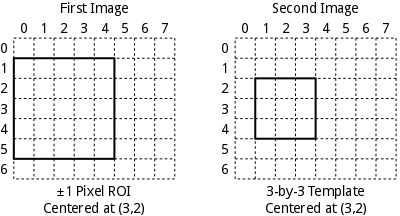
Another example of a different part of the problem space
is represnted by basic block matching used in stereo
vision applications to generate a disparity map. As shown
in the image below, a large number of small ROIs are
defined around every pixel in one image (left). A template
unique to that ROI is extracted from the other image
(right) centered around the corresponding pixel. In
contrast to linear image filter, we have a large number of
relativley small ROIs (often with purely horizontal
search) and many unique templates.
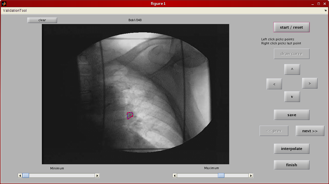
Large-Template Tracking Application
The first application that we have targetted for
acceleration is a tumor tracking application developed
by Cui et al. A screenshot of the
application is shown below.
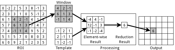
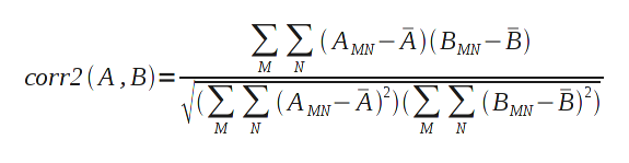
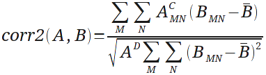
The application uses multiple fixed templates with
Person's correlation as a similarity score. Pearson's
correlation is performed by
the corr2() function in
the MATLAB
Image Processing Toolbox, and is represented by the
following equation:
The A
and B in
the above equation represent matrix mean. So, for a given
template, A, the contribution to the denominator is fixed
for all sliding window positions, as is the templates
contribution to the denominator. Since the templates are
calculated once and used for the duration of a session,
these parts of the corr2()
function can be computed once and reused, reducing the
computation to the following:
It should be noted that the value
of B, the
frame data mean, depends on the current window
location. This aspect of the computation prevents an
efficient frequency domain implementation.
Data Sets
We have been working with a number of sample data sets,
which are summarized in the following table:
The sizes of the templates are specified by hand and may
vary based on tumor size as well as human factors. As a
result, the range of template sizes varies
significantly. They are also much larger than the
templates usually considered for GPU-accelerated sliding
window applications. Another difference is that while
there is only one ROI per frame, like linear image
filtering, the ROI and corresponding search space is much
smaller. These factors place this tumor tracking
application into a different part of the sliding window
problem space.
Problems Mapping to CUDA
There are a couple problems that arrise when considering a
mapping of this problem into CUDA. The first has to do
with data placement and memory selection. A common
approach for mapping sliding window operations is to
assign one or more template positions to a thread. The
threads within a block will be assigned adjacent sets of
one or more window positions per thread. This works well
with the shared memory in NVIDIA GPUs, as adjacent window
positions require all of the same underlying image data
with the exception of one row or column. Loading the union
of needed image data into shared memory and processing out
of shared memory significantly decreases the demands on
global memory and keeps frequently accessed values in the
SM. In general, proper usage of shared memory is crucial
for GPGPU performance.
A problem with this approach is that the template sizes in
our data sets are larger than usually considered. Only the
template and ROI for the smallest patient will fit into
shared memory for 1.x devices.
A second issue with mapping this tracking application to
CUDA is where to generate parallelism. There are only a
few templates. Assuming streaming operation only one ROI
is resident at a time, and for each ROI the search space
is small - 95 to 703 search positions.
Tiled Template
Our solution to these problems is to break the large
templates into tiles and process the tiles
separately. Since the outer loops of both the numerator
and denominator of the corr2()
function are summations, the tiles can be processed
independently. With each tile mapped to a thread block,
this approach generates more sources for independent
parallelism and reduces the working set size for shared
memory. A second step is then required to combine the
contributions of each tile to produce the final result.
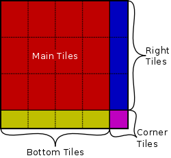
With tiles mapped to the CUDA grid this approach scales to
arbitrarily large template sizes, limited only by the
limitations on grid size (65,536 in each direction). As
can be seen in the above image, a tile size that executes
efficiently on a target GPU may not cover an arbitrary
template size with an integer number of tiles. In these
cases, there will be leftover tiles on the right and/or
bottom. When both right and bottom leftover tiles are
present, there will also be a corner tile. The defintion
of the corr2() function, with
the matrix mean subtraction, complicates the padding.
Our current implementation only adjusts one dimension for
these edge case tiles. Only the width of the tile will be
adjusted for the tiles on the right, and only the height
of the tile will be adjusted on the bottom. Depending on
the main tile size chosen, this can affect the number and
type of leftover tiles. As an example of this, the
following table shows various tile sizes and counts for
Patient 4 (156×116 pixel template size) when
different main tile sizes are selected:
More addition is used to combine the contributions of each
tile in a reduction kernel. The intermediate data is
grouped by tile. Since each tile is shifted over the same
shift area regardless of its dimensions, the main, left,
bottom, and corner tiles have the same data layout. This
attribute results in a relatively simple and fully
coalesced reduction kernel.
The frame data averages, frame data contribution to the
denominator, and the numerator are performed in order each
each consists of the two stages described above: a tiled
summation step and then a reduction. A simple element-wise
kernel is used to implement the final fraction.
Current Performance
For the six data sets above, arbitrary tile sizes ranging
from 4×4 to 16×16 were benchmarked. The GPU
results were compared with reference MATLAB and
multi-threaded C implementations of the tumor tracking
application. The hardware used for these results was an
Intel Xeon W3580 (4 i7 cores @ 3.33 GHz and 6 MB
L2 cache) and a NVIDIA Tesla C1060. The machine was
running Ubuntu 10.04 64-bit, MATLAB R2010a and CUDA 3.1.
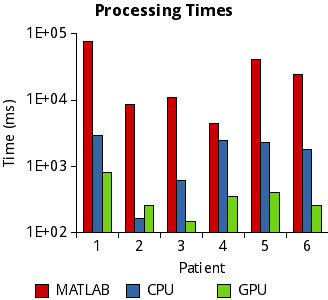
The graph below shows the total application run times for
the data sets, including data transfer. The tiled GPU
implementation achieves good performance across the data
sets. The only scenario where the GPU is not faster than
the multi-threaded CPU implementation is for Patient 2,
where the small size of the template combined with the
small search area prevent enough parallelism to be
generated for efficient GPU execution, even when using
small templates.
The following table presents the best speedup over the
multi-threaded CPU version combined with which of the
arbitrary main tile sizes achieved the best performance:
As can be seen in the graph below, the numerator dominates
the GPU version runtime. This is because the numerator is
the most complicated step as well as the fact that it has
to be performed for each template. In contrast, the frame
data averages and denominator contribution can be computed
only once per frame and are applied to each template.
Ongoing Work
The tiled implementation described above is being used as
the basis for further exploration of the issues
surrounding adapatable CUDA implementations. Ongoing
research includes augmenting the tiled template GPU
kernels to handle arbitrary shift areas, examining the
proper dimensions for parameterizaiton of a sliding window
library element for both problem and hardware target
adaptation, and examining the benefits of problem-specific
kernel compilation.
Shift Area Tiling
The results described above used a maximum thread count of
192 threads per block. The benchmakred implementation uses
one thread per window location, so any time a patient data
set consisted of more than 192 search positions per ROI,
multiple kernel calls were used. Furthermore, a maximum of
512 (for 1.x GPUs) threads per block is possible for a
kernel launch, and one of the patient data sets consists
of 703 search positions. In general, between 128 and 256
threads per block is a desirable target for CUDA
applications.
To eliminate the need for multiple kernel launches and
enable the GPU implementation to handle sliding window
problem instances with much larger search areas, we are
working on tiling the search space in manner similar to
that used for tiling the template. This would allow a
single implementation to cover problems with large
templates, like the tumor tracking application above, as
well as problems with a large search space, such as linear
image filtering. Tiling of the search space can take the
form of assigning multiple shift positions to each thread
as well as launching a larger grid with more thread blocks
to cover the extra search area.
Parameterization
Besides the parameters related to the sliding window
problem, the current GPU impelentation introduces two
implementation parameters: tile size and shift area per
block. These parameters allow the implementation to trade
limited block resources for the less constrained grid
dimensions.
In general, these types of tradeoffs can be used to help
adjust implementations to different execution
hardware. For example, adjusting the tile size trades
shared memory requirements for grid area. The shift area
assigned to each block trades grid area for both thread
count per block and shared memory requirements. With these
implementation parameters, for example, the data working set
size can be adjusted to the target GPUs shared memory size
(16 KB or 48 KB) and maximum threads per block
count (512 vs 1024).
Obtaining knowledge and generating heuristics for
selecting the values for implementation parameters for an
incoming problem instance is one of the main goals of our
ongoing work. We would also like to determine which target
hardware parameters are relevant for making these
decisions, or if some type of empirical benchmarking
search is necessary.
Problem-Specific Kernel Compilation
While not mentioned in the discussion of the tiled
template implementation, our GPU kernels are compiled at run
time specifically for the current problem. As it stands,
run time compilation is used to compile in up to four
custom copies of the main computation loops, one for each
needed tile size. This allows for full unrolling of the
loops, and important GPU compile-time optimization that is
not avaiable when the kernel is compiled once before the
template dimensions have been determined. Loops for the
reductions can also be unrolled. When main tile sizes that
are powers of two are selected, the compiler can perform
strength reduction on modulus and division operations
converting them to bitwise operations.
This approach eliminates overheads assocated with handling
the edge cases tiles and their random tile sizes. A good
example of this phenomenon occurs for Patient 4. While a
4×4 pixel main tile
size eliminates edge-case
tiles, the best performance was achieved with
a 16×10 pixel main
templatesize.
While the current runtime compilation uses appear to be
beneficial, particularly in terms of reducing per thread
register usage, we are currently exploring greater use of
problem-specific kernel compilation. This can be of
particular help when dealing with adaptable GPU
kernels. GPUs tend not to deal well with control heavy
code (adaptable code), as things like thread divergence
and loops have relatively high overheads. By adding shift
area tiling, we are also mapping an increasing number of
parameters into the fixed CUDA thread hierarchy requiring
an increasing number of non-compute instructions used to
have each thread calculate its offest into the problem
space. Compiling custom kernels for each problem helps to
sidestep some of these issues by moving repeated expensive
runtime evaluation to compile time.
In addition, this approach also has some hardware target
adaptability benefits. For example, CUDA C supports C++
style templates that can be used to select
between *
and __[u]mul24() for integer
arithmetic depending on the target. Any additional
knowledge the compiler has about the target can also be
applied.
An area of interest is exploring and analyzing the
benefits of run time kernel compilation. We would like to
quantify the benefits, if any, beyond annectdotal
experiences of loop unrolling and register usage
reduction. In addition, we would like to know the limits
of this approach: When should parameters be compiled into
a kernel? When should customized instances be included?
How much can be done in terms of hardware adaptability?
Can we swap out the per-window location processing to
reduce redundant code?
Particle Image Velocimetry
The tumor tracking application has provided a starting
point for this work and a represents a unique part of the
problem space. In order expand problem space coverage and
help us derive heuristics for automatic configuration
selection and parameterization, we are currently looking
at particle image velocimetry (PIV).
PIV is
an active
area of interest for our group and has been studied
for FPGA implementation. Our current
formulation of the problem uses multiple non-adjacent ROIs
per frame with a small to medium search. This places the
problem in a different part of the sliding window problem
space.